In physics and mathematics, in the area of dynamical systems, an elastic pendulum[1][2] (also called spring pendulum[3][4] or swinging spring) is a physical system where a piece of mass is connected to a spring so that the resulting motion contains elements of both a simple pendulum and a one-dimensional spring-mass system.[2] The system exhibits chaotic behaviour and is sensitive to initial conditions.[2] The motion of an elastic pendulum is governed by a set of coupled ordinary differential equations.
Analysis and interpretation
The system is much more complex than a simple pendulum, as the properties of the spring add an extra dimension of freedom to the system. For example, when the spring compresses, the shorter radius causes the spring to move faster due to the conservation of angular momentum. It is also possible that the spring has a range that is overtaken by the motion of the pendulum, making it practically neutral to the motion of the pendulum.
Lagrangian
The spring has the rest length 


The Lagrangian 

where 

See. Hooke's law is the potential energy of the spring itself:

where 
The potential energy from gravity, on the other hand, is determined by the height of the mass. For a given angle and displacement, the potential energy is:

where 
The kinetic energy is given by:

where 

So the Lagrangian becomes:[1]

![{\displaystyle L[x,{\dot {x}},\theta ,{\dot {\theta }}]={\frac {1}{2}}m({\dot {x}}^{2}+(l_{0}+x)^{2}{\dot {\theta }}^{2})-{\frac {1}{2}}kx^{2}+gm(l_{0}+x)\cos \theta }](https://wikimedia.org/api/rest_v1/media/math/render/svg/51844c7831278ecdfb989c51b95d780d91a0fa1f)
Equations of motion
With two degrees of freedom, for


For


And for


The elastic pendulum is now described with two coupled ordinary differential equations. These can be solved numerically. Furthermore, one can use analytical methods to study the intriguing phenomenon of order-chaos-order[6] in this system.
In physics and mathematics, in the area of dynamical systems, an elastic pendulum[1][2] (also called spring pendulum[3][4] or swinging spring) is a physical system where a piece of mass is connected to a spring so that the resulting motion contains elements of both a simple pendulum and a one-dimensional spring-mass system.[2] The system exhibits chaotic behaviour and is sensitive to initial conditions.[2] The motion of an elastic pendulum is governed by a set of coupled ordinary differential equations.
Analysis and interpretation Edit
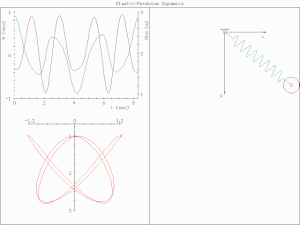
2 DOF elastic pendulum with polar coordinate plots. [5]
The system is much more complex than a simple pendulum, as the properties of the spring add an extra dimension of freedom to the system. For example, when the spring compresses, the shorter radius causes the spring to move faster due to the conservation of angular momentum. It is also possible that the spring has a range that is overtaken by the motion of the pendulum, making it practically neutral to the motion of the pendulum.
Lagrangian Edit
The spring has the rest length {\displaystyle l_{0}}l_0 and can be stretched to length {\displaystyle x}x. The angle of oscillation of the pendulum is {\displaystyle \theta }\theta .
The Lagrangian {\displaystyle L}L is:
{\displaystyle L=T-V}L=T-V
where {\displaystyle T}T is the kinetic energy and {\displaystyle V}V is the potential energy.
See. Hooke's law is the potential energy of the spring itself:
{\displaystyle V_{k}={\frac {1}{2}}kx^{2}}{\displaystyle V_{k}={\frac {1}{2}}kx^{2}}
where {\displaystyle k}k is the spring constant.
The potential energy from gravity, on the other hand, is determined by the height of the mass. For a given angle and displacement, the potential energy is:
{\displaystyle V_{g}=-gm(l_{0}+x)\cos \theta }{\displaystyle V_{g}=-gm(l_{0}+x)\cos \theta }
where {\displaystyle g}g is the gravitational acceleration.
The kinetic energy is given by:
{\displaystyle T={\frac {1}{2}}mv^{2}}{\displaystyle T={\frac {1}{2}}mv^{2}}
where {\displaystyle v}v is the velocity of the mass. To relate {\displaystyle v}v to the other variables, the velocity is written as a combination of a movement along and perpendicular to the spring:
{\displaystyle T={\frac {1}{2}}m({\dot {x}}^{2}+(l_{0}+x)^{2}{\dot {\theta }}^{2})}{\displaystyle T={\frac {1}{2}}m({\dot {x}}^{2}+(l_{0}+x)^{2}{\dot {\theta }}^{2})}
So the Lagrangian becomes:[1]
{\displaystyle L=T-V_{k}-V_{g}}{\displaystyle L=T-V_{k}-V_{g}}
{\displaystyle L[x,{\dot {x}},\theta ,{\dot {\theta }}]={\frac {1}{2}}m({\dot {x}}^{2}+(l_{0}+x)^{2}{\dot {\theta }}^{2})-{\frac {1}{2}}kx^{2}+gm(l_{0}+x)\cos \theta }{\displaystyle L[x,{\dot {x}},\theta ,{\dot {\theta }}]={\frac {1}{2}}m({\dot {x}}^{2}+(l_{0}+x)^{2}{\dot {\theta }}^{2})-{\frac {1}{2}}kx^{2}+gm(l_{0}+x)\cos \theta }
Equations of motion Edit
With two degrees of freedom, for {\displaystyle x}x and {\displaystyle \theta }\theta , the equations of motion can be found using two Euler-Lagrange equations:
{\displaystyle {\partial L \over \partial x}-{\operatorname {d} \over \operatorname {d} t}{\partial L \over \partial {\dot {x}}}=0}{\displaystyle {\partial L \over \partial x}-{\operatorname {d} \over \operatorname {d} t}{\partial L \over \partial {\dot {x}}}=0}
{\displaystyle {\partial L \over \partial \theta }-{\operatorname {d} \over \operatorname {d} t}{\partial L \over \partial {\dot {\theta }}}=0}{\displaystyle {\partial L \over \partial \theta }-{\operatorname {d} \over \operatorname {d} t}{\partial L \over \partial {\dot {\theta }}}=0}
For {\displaystyle x}x:[1]
{\displaystyle m(l_{0}+x){\dot {\theta }}^{2}-kx+gm\cos \theta -m{\ddot {x}}=0}{\displaystyle m(l_{0}+x){\dot {\theta }}^{2}-kx+gm\cos \theta -m{\ddot {x}}=0}
{\displaystyle {\ddot {x}}}{\ddot x} isolated:
{\displaystyle {\ddot {x}}=(l_{0}+x){\dot {\theta }}^{2}-{\frac {k}{m}}x+g\cos \theta }{\displaystyle {\ddot {x}}=(l_{0}+x){\dot {\theta }}^{2}-{\frac {k}{m}}x+g\cos \theta }
And for {\displaystyle \theta }\theta :[1]
{\displaystyle -gm(l_{0}+x)\sin \theta -m(l_{0}+x)^{2}{\ddot {\theta }}-2m(l_{0}+x){\dot {x}}{\dot {\theta }}=0}{\displaystyle -gm(l_{0}+x)\sin \theta -m(l_{0}+x)^{2}{\ddot {\theta }}-2m(l_{0}+x){\dot {x}}{\dot {\theta }}=0}
{\displaystyle {\ddot {\theta }}}{\displaystyle {\ddot {\theta }}} isolated:
{\displaystyle {\ddot {\theta }}=-{\frac {g}{l_{0}+x}}\sin \theta -{\frac {2{\dot {x}}}{l_{0}+x}}{\dot {\theta }}}{\displaystyle {\ddot {\theta }}=-{\frac {g}{l_{0}+x}}\sin \theta -{\frac {2{\dot {x}}}{l_{0}+x}}{\dot {\theta }}}
The elastic pendulum is now described with two coupled ordinary differential equations. These can be solved numerically. Furthermore, one can use analytical methods to study the intriguing phenomenon of order-chaos-order[6] in this system
| This article uses material from the Wikipedia article Metasyntactic variable, which is released under the Creative Commons Attribution-ShareAlike 3.0 Unported License. |
.